Fig 224. Projectile at near-sonic speed
Table of Content
$$ \vcenter{M = 0.978} $$
$$ \vcenter{M = 0.990} $$ “Still closer to the speed of sound, the shock-wave pattern of the preceding pages had spread laterally to great distances. These two photographs are from the same firing, so that the second one was actually taken earlier in the trajectory” Photographs by A. C. Charters, in von Kármán 1947
Theory #
These simulations are part of a series together with figure 223 and figure 253 all done in transonic flow. The shockwaves and convex corner flow around the bullet make for switches between subsonic and supersonic flow. Here the main challenges of simulating transonic flow are discussed.
The Transonic flow problem #
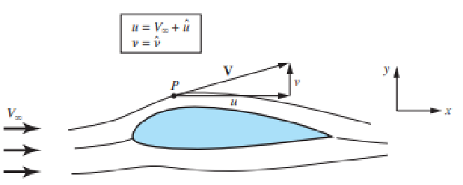
For transonic flow the change in velocity around Mach 1 complicated early CFD computations. This can be seen in the non-linear perturbation velocity potential equation for transonic flow, which was used back in the day and follows from the definition of the velocity potential \(\phi\) for 2D:
$$
\mathbf{V} = \nabla \phi \\
u = V_{\infty} + \hat{u} \\
v = \hat{v}
$$
With u and v being cartesian velocity components in x and y direction respectively, V being the velocity magnitude, \(V_{\infty}\) flow field velocity and \(\hat{u}\) and \(\hat{v}\) being velocity perturbations (increments).
Using \(\phi\) to obtain one equation that represents a combination of the continuity, momentum and energy equations is useful to use one governing equation with one unknown. This creates the final equation:
$$ (1-M_{\infty}^2) \frac{\partial^2 \hat{\phi}}{\partial x^2} + \frac{ \partial^2 \hat{\phi}}{\partial y^2} = M_{\infty}^2 [(\gamma + 1)\frac{\partial \hat{\phi}}{\partial x}\frac{1}{V_{\infty}}] \frac{\partial^2 \hat{\phi}}{\partial x^2} $$ It is important to note here that this equation approximates the physics of a steady, compressible, inviscid 2D flow. The important point here is the factor (\(1-M_{\infty}^2\)), which will be higher than 0 in subsonic flow and lower than 0 for supersonic flow and result in a different form of partial differential equation. In supersonic flow, it is a hyperbolic partial differential equation while in subsonic it is an elliptic partial differential equation, which is a big difference in math type. This shows a big difference in physics between subsonic and supersonic flow.
This equation was used in the earliest transonic CFD simulations. Later Euler equations were used, which predict shockwaves pretty well, but do not fare well in transonic flow due to shock wave interaction with the boundary layer, which needs viscosity. For a comparison a look can be taken at Figure 223. The current state of the art for transonic flow is solving the Navier-Stokes equations with the viscous term. Here the turbulence model frequently being the Achilles heel of these complicated calculations [1].
Transonic buffet #
In transonic flow, the interactions between shock waves and separated shear layers result in self-sustained low-frequency oscillations of the shock wave also called transonic buffet. Some aspects of these oscillations are still incomprehensible [2]. A transient computational setup with LES is needed to show these oscillations and comes at a high cost. The steady-state simulations done estimate the average position.
Numerical dissipation #
CFD simulations currently in transonic flow are very sensitive to artificial dissipation characteristics of the computational fluid algorithm. With a bad algorithm problems such as difficult convergence, poor reliability and difficulty to accurately simulate shock position will occur [3].
Numerical dissipation is an artificial effect that is introduced when solving the governing equations, which acts as an unnatural damping of the variables at play. This with as main goal to damp oscillations and smooth out high-frequency noise and thus stabilizing the solution ensuring convergence [4]. Turbulence models and mesh refinement around areas with steep gradients lower the amount of numerical dissipation needed.
Simulation & Visualization #
About the simulation and visualization can be read in figure 253.
References #
- [1] Fundamentals-of-aerodynamics-6-Edition.pdf
- [2] https://www.sciencedirect.com/science/article/pii/S0376042117300271
- [3] https://ieeexplore.ieee.org/document/10082199
- [4] https://www.nas.nasa.gov/assets/nas/pdf/ams/2018/introtocfd/Intro2CFD_Lecture7_Zingg.pdf)