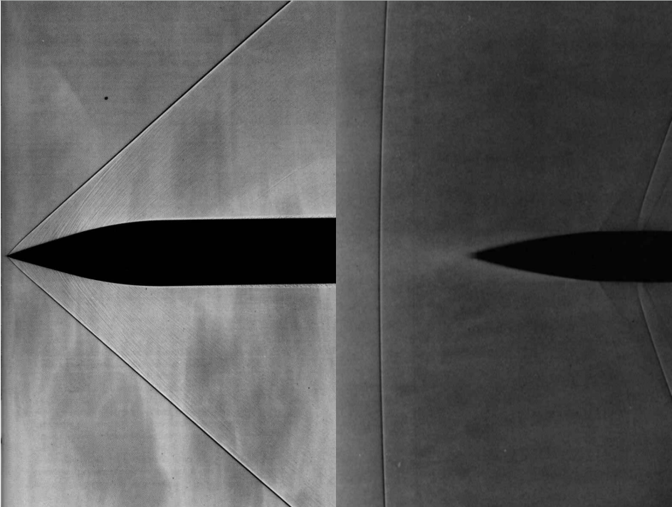
Fig 253. Projectile at M=1.015

Table of Content

“The model artillery shell of figures 223 and 224 is shown here still earlier in its trajectory, when it is flying at a slightly supersonic speed. A detached bow wave precedes it, and the distant field is quite different, but the pattern near the body is almost identical to that shown in figure 224 for a slightly subsonic speed. This illustrates how the near field is ‘frozen’ as the free-stream Mach number passes through unity.” Photograph by A. C. Charters

Theory>

Theory #

Shockwaves>

Shockwaves #

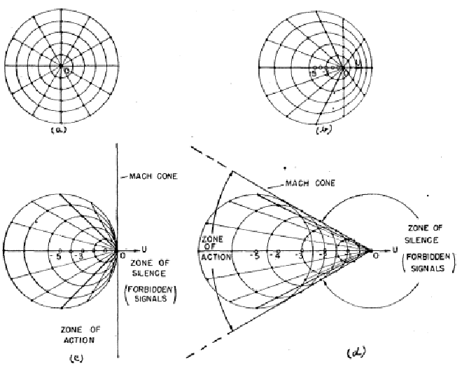
Shockwaves appear with flows that reach velocities higher than 1 Mach, the speed of sound through the medium. This is due to that pressure changes in a medium are diffused at the speed of sound of that medium. When a disturbance makes flow streamlines with a higher Mach number than 1 turn in on itself, the disturbance travels faster than the pressure diffusion and is unable to send a ‘signal’ to the upstream flow. This is while in subsonic flow the particles in front of the object are already ‘informed’ by pressure changes in front of the disturbance and move out of the way. In supersonic flow, the particles do not move out of the way and as the disturbance arrives nanoscale molecular collisions find place.

When a body moves through a fluid at supersonic speed it creates a pressure front moving at supersonic speed pushing on the air. This pushing creates a high-pressure region resulting in a very thin shockwave with abrupt changes in flow properties, with an increase in potential energy at the cost of kinetic energy. The density, pressure, and temperature increase, while the velocity decreases [1].

The angle of the shockwave of a particle is decided by the speed of sound as the pressure signal relative to the particle travels in all directions at sound velocity minus relative flight velocity depicted in the following figure:

point source moving in a compressible fluid. — Point source moving in a compressible fluid. a, stationary. b, half the speed of sound. c, at the speed of sound. d, twice speed of sound [2]

The leading curved shockwave is called a detached shock or bow shock. This happens as the change in flow direction through a shockwave is too small and the fluid cannot move out of the way, as is the case with a blunt body [3]. The distance between the body and the detached shock is based on the flow velocity and the body shape. A lower velocity and a wider body are factors that make the distance between the detached shock and the body larger [2].

oblique vs bow shock. — Left oblique shock (figure 261), right bow shock

The detached shockwave creates a subsonic flow in front of the body. Further from the object the detached shockwave gets a lower bending radius and becomes oblique.

Transonic convex corner flow>

Transonic convex corner flow #

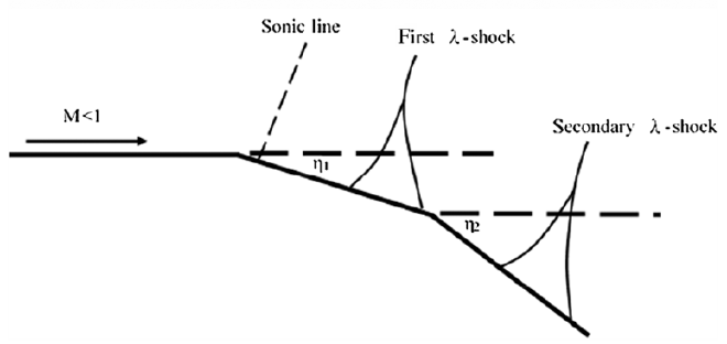
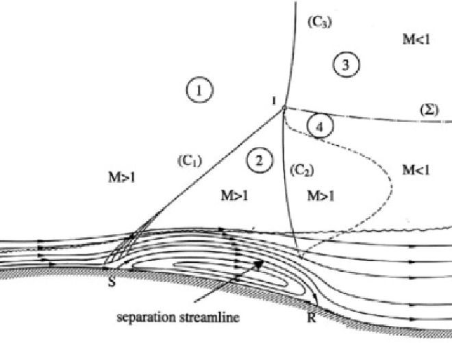
Supersonic flow going around a convex corner is known as a Prandtl-Meyer expansion, which increases the dynamic properties and decreases the static properties as the “opposite” of a shockwave. In transonic flow, the flow region of this experiment, it is a bit different due to the flow arriving at the convex corner being subsonic. The flow accelerates around the corner to become supersonic and undergoes extra acceleration in the expansion Prandtl-Meyer fan, downstream shockwaves find place.

biconvex-corner flows. — Schematic drawing for biconvex-corner flows with \({\lambda}\)-shock waves [4]

This results in a so-called \({\lambda}\)-shock structure, which is a prime example of shock wave boundary interaction. The first leg is where shock-induced boundary layer separation takes place, the second leg is near the reattachment location. Boundary layer separation can be attributed to the adverse pressure gradient, the static pressure increases over the boundary layer, due to the shockwave. The increase in potential energy is big enough to reduce the boundary velocity enough to reverse it creating flow separation.

For more information on detached flow visit Figure 42

Simulation>

Simulation #

Domain>

Domain #

While making the 2D domain the shape was traced from the original image, and small details on the body were added based on the shock- and expansion waves. For example, a small increase in diameter at the middle of the shell is found based on expansion waves.

Further downstream of the body, figures 223 and 224 show biconvex-corner flows for this shell model, which was tried to model correctly with iterations, where in the end a small curve showed the best result. There is suspected to be a hole based on images of different types of 155mm artillery shells and iterating over CFD simulations. CFD experiments have shown that the cutout significantly lowers the height of the back \({\lambda}\)-shock in high subsonic velocities, mainly in Figure 223 and Figure 224. The detached shock distance is still to close to the shell, after iterations a small dimple in the nose seemed to move the shockwave a bit more upstream, however the real bow shock location was not achieved.

The domain is made for an axisymmetric simulation by using an axis boundary at the x-axis, a no-slip wall boundary condition for the object, and a far-field boundary for the other three boundaries. Gauge pressure and temperature have been found irrelevant to the shape of the waves, as the temperature influences the speed of sound and only the Mach number is used as input. Pressure

Meshing>

Meshing #

The start mesh is a quadrilateral hybrid mesh of 0.0055 m, which is quite small to have a better discretization of the problem before adaptive refinement. Hybrid meshes were easy to use while iterating a complex shape, but pay a price in memory, execution speed, and numerical convergence compared to a well-structured mesh. Another downside is that the mesh has quite a high boundary layer with a loss of detail in this region. After running the simulation, the mesh is refined by using ansys adaptive refinement tools around density changes, to capture the shockwaves with higher detail, and refined again around the shell body to better caption shock wave boundary layer interaction. More refinement was not possible at the risk of convergence as the Ansys tool only divides one quadrilateral element into four which is bad for the volume ratio between cells [6].

Fluid model>

Fluid model #

The solver type used is density-based, as it gives better accuracy for high-speed flow with shockwaves than pressure-based solvers. Because of the compressible flow used in calculations for shockwaves the ideal gas law is used for air, as an extra equation on top of the compressible Navier-Stokes equations to solve for four unknowns: Density, pressure, velocity, and energy or enthalpy.

For viscosity, the realizable k-epsilon model is used, as viscous forces are rarely dominant in the Navier-Stokes equations due to high velocity but are important to capture shock wave boundary layer interaction. More on viscosity models can be found in Figure 47. Further, Sutherland’s Law is used for the viscosity changes of the air due to temperature changes.

Visualization>

Visualization #

The original image is a spark photograph in which the different densities around the artillery shell act as lenses and refract the light. That is why on the original experiment the shock waves’ colour went from dark to light, due to the big density change and thus big change in refraction.

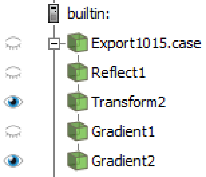
Paraview is used for visualization, using two gradient filters on density to create a second-order gradient in the horizontal direction. This is to create the dark-to-white shockwaves in the original image. The gradient filter has some opacity, and the colour scale values have been altered to fit the replicated image. The Transform filter is used to rotate the object around the z-axis to fit the original image.

References>